DemoSpectralClustering

a Matlab GUI to explore spectral clustering and the influence of different similarity graphs

by Matthias Hein and Ulrike von Luxburg

PURPOSE

DemoSpectralClustering: In this demo, we would like to show how (normalized) spectral clustering behaves for different kinds of neighborhood graphs. In particular, we want to explore how the first eigenvectors of the graph Laplacian and the resulting low-dimensional embeddings react for different choices of neighborhood graphs.

TUTORIAL

DemoSpectralClustering has been used for teaching purposes at the Machine Learning Summer School 2007 in Tuebingen, Germany. The tutorial which is based on DemoSpectralClustering introduces the theoretical foundations of spectral clustering as well as given practical hints for spectral clustering using behavior on toy datasets.

Download tutorial on spectral clustering   

SCREENSHOT OF DemoSimilarityGraphs

PANELS IN DemoSpectralClustering

This demo implements normalized spectral clustering, using the eigenvectors of the random walk Laplacian L_rw = D^{-1} (D - S). The eigenvectors are used to map each data point i to the new representation (v_1i, v_2i, ..., v_ki), which yields an embedding of the data points into Euclidean space. The final clustering is done using k-means clustering in the new representation. Of course there are many other variants of spectral clustering which we did not incorporate in the demo. For a survey of some of them see the overview paper A tutorial on spectral clustering .

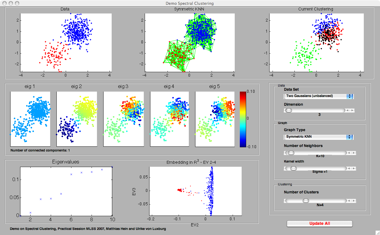
• The first row contains three plots, which are more or less self-explanatory: the first plot shows the data set, the second plot the current similarity graph. Both of those plots coincide with the corresponding plots in DemoSimilarityGraphs. The third plot shows the clustering of data obtained using spectral clustering.
• The eigenvector plots (second row): here we plot the first 5 eigenvectors (in subfigures 1 to 5, from left to right) of the Laplacian L_rw. Those eigenvectors are used to construct the embedding used in spectral clustering. If v = (v_1, ..., v_n)' denotes a particular eigenvector, the corresponding eigenvector plot shows the data points x_i, color-coded by the entry v_i of the eigenvector. Ideally, the eigenvectors should be more or less constant on the clusters. Note that the color-scale is the same in all five eigenvector plots, as shown in the colorbar to the right.
• The eigenvalues (third row): here we plot the 10 smallest eigenvalues of L_rw, ordered by size. In detail, we plot i versus lambda_i, where lambda_i is the i-th smallest eigenvalue of L_rw.
• Embedding (third row): this plot shows the embedding used in spectral clustering. We plot the embedding realized by the first three informative eigenvectors. Note that if the graph is connected, then the first eigenvector is the constant 1 vector, which we discard in the plot. We then plot the points (v_2i, v_3i, v_4i) where v_ji denotes the i-th entry in eigenvector j. In case the graph is disconnected, the first eigenvector is not constant. In this case we plot (v_1i, v_2i, v_3i). Note that by clicking on the plot and moving the mouse, one can rotate this plot to get a 3d-impression.